





If you’d rather listen than read, feel free to play the audio file below for the rest of this article.
What Is Power Factor? A Precise Definition
Power factor is the ratio of active power doing useful work to apparent power drawn from the supply. It is a dimensionless number between 0 and 1, often shown as a decimal or percentage. The symbol PF describes how effectively a circuit converts supplied electrical energy into productive output.
A value of 1.0 — known as unity power factor — occurs only in purely resistive circuits. Every volt-ampere then performs work. By contrast, values below unity mean part of the apparent power circulates as reactive energy without driving any load.
This behavior arises because voltage and current in AC circuits can fall out of phase. Inductors delay current; capacitors advance it. Therefore, the phase angle (φ) widens, and cos(φ) — the circuit power factor — falls.
Mathematically, PF = cos(φ). Hence, the term “cos phi electrical” frequently appears in European literature. Engineers reading energy analyzers see both notations interchangeably.
Visit this page to learn more about the specifications, applications, and related details.
Understanding this ratio becomes far easier once the underlying theory is clear, so review our guide to electrical fundamentals before moving deeper into reactive concepts.
The Three Types of Power in AC Systems
Three quantities govern every AC power system, and each plays a distinct role in determining the real power to apparent power ratio at the supply terminals. Engineers must distinguish them clearly before sizing equipment or planning correction measures.
Active power performs useful work — spinning shafts, producing heat, illuminating fixtures. Reactive power, by contrast, oscillates between source and load to sustain magnetic and electric fields. Apparent power is the vector sum of both and represents what the supply infrastructure must physically carry.
Misreading these quantities causes expensive errors. For example, sizing a transformer on kW rather than kVA leaves no headroom for reactive current. Furthermore, many tariffs penalize excess kVA demand even when the kWh figure remains modest.
The following subsections define each quantity precisely. A summary table afterwards consolidates the relationship for quick reference.
This external page provides additional insights that may help with your evaluation.
Active Power (Real Power) — P
Active power, measured in watts or kilowatts, is the component a load actually consumes. It drives motor shafts, heats elements, and lights fixtures. Utilities bill this energy in kWh, and it represents the productive output every facility ultimately wants to maximize.
This website offers useful supporting information for understanding the subject more clearly.
Reactive Power — Q
Reactive power, measured in VAR or kVAR, exchanges between source and reactive components — inductors and capacitors. It performs no work yet remains essential for establishing magnetic fields. However, this circulating current still travels through conductors and therefore contributes to losses and capacity limits.
You can check this page for more examples, explanations, and related technical resources.
Apparent Power — S
Apparent power, measured in VA or kVA, is the vector sum of active and reactive components. Utility transformers, cables, and switchgear are rated on kVA, not kW. Consequently, a poor real-power-to-apparent-power ratio forces facilities to install larger infrastructure than the productive load alone would demand.
| Power Type | Symbol | Unit | What It Represents | Does Useful Work? |
|---|---|---|---|---|
| Active Power | P | W / kW | Power Converted to Useful Output | Yes |
| Reactive Power | Q | VAR / kVAR | Power Exchanged with Reactive Components | No |
| Apparent Power | S | VA / kVA | Total Power Supplied; Vector Sum of P and Q | Partially |
For updated product, service, or technical information, review the source website directly.
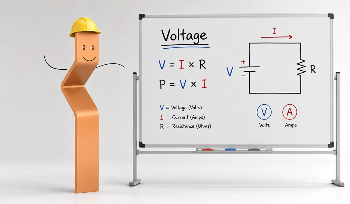
Engineers who want a firmer grounding in these quantities should first revisit how voltage, current and resistance interact, because every power calculation rests on those variables.
The Power Factor Formula
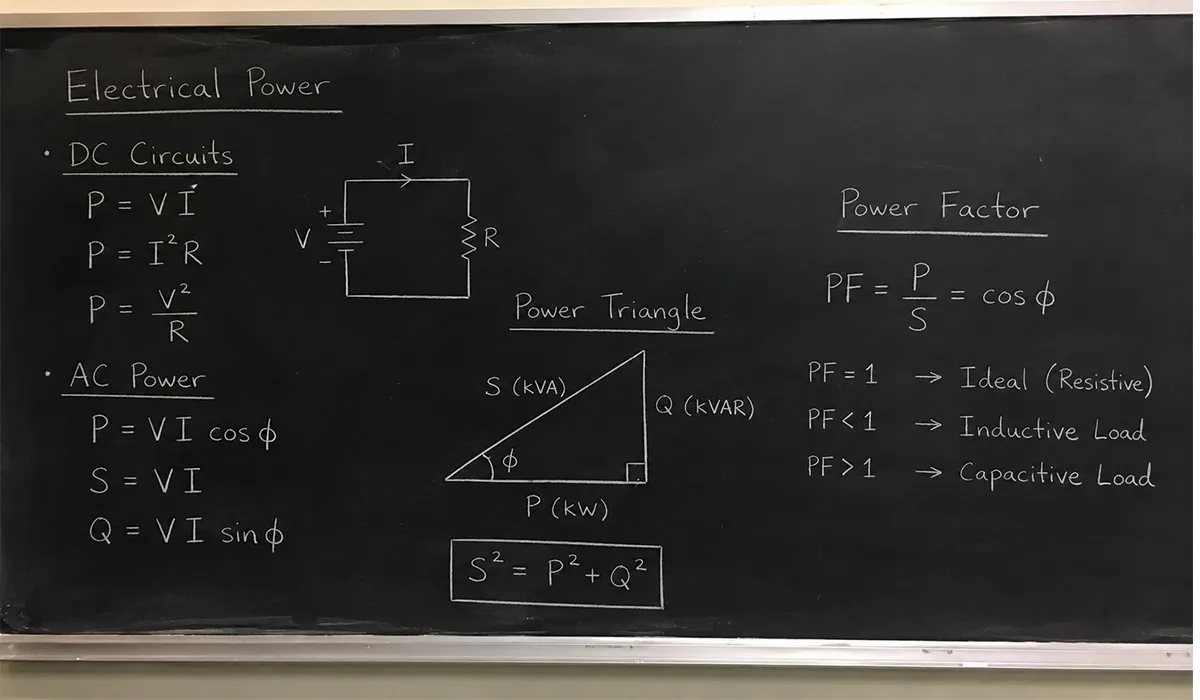
Engineers express the power factor formula through two equivalent relationships. The fundamental form is PF = P ÷ S, where P is active power in kW and S is apparent power in kVA. Equivalently, PF = cos(φ), where φ is the phase angle between voltage and current.
From these two expressions, every other useful relationship follows directly. For instance, active power equals V × I × cos(φ) in single-phase systems. Likewise, reactive power equals S × sin(φ). The phase angle itself comes from φ = arccos(PF).
In practice, technicians rarely calculate values by hand. Modern energy analysers compute them continuously and log trends across operating cycles. Nevertheless, understanding the formula is essential for sizing capacitor banks, evaluating correction proposals, and interpreting utility tariffs.
The reference table below consolidates all working forms used during system design, equipment selection, and audit calculations.
| To Calculate | Formula | Units |
|---|---|---|
| Power Factor | PF = P ÷ S | Dimensionless |
| Power Factor | PF = cos(φ) | Dimensionless |
| Active Power | P = S × PF | W or kW |
| Active Power | P = V × I × cos(φ) | W or kW |
| Apparent Power | S = P ÷ PF | VA or kVA |
| Apparent Power | S = V × I | VA or kVA |
| Reactive Power | Q = S × sin(φ) | VAR or kVAR |
| Phase Angle | φ = arccos(PF) | Degrees |
Worked Example — Calculating Power Factor
A 230 V single-phase line delivers 8 A to an inductive load. The meter reads 1,472 W. Then S = 230 × 8 = 1,840 VA, and PF = 1,472 ÷ 1,840 = 0.80. Therefore the load uses 80% of supplied capacity productively. Likewise, a 250 kVA service operating at 0.92 yields P = 230 kW and Q ≈ 98 kVAR.
The Power Triangle: Visualizing the Relationship Between P, Q, and S
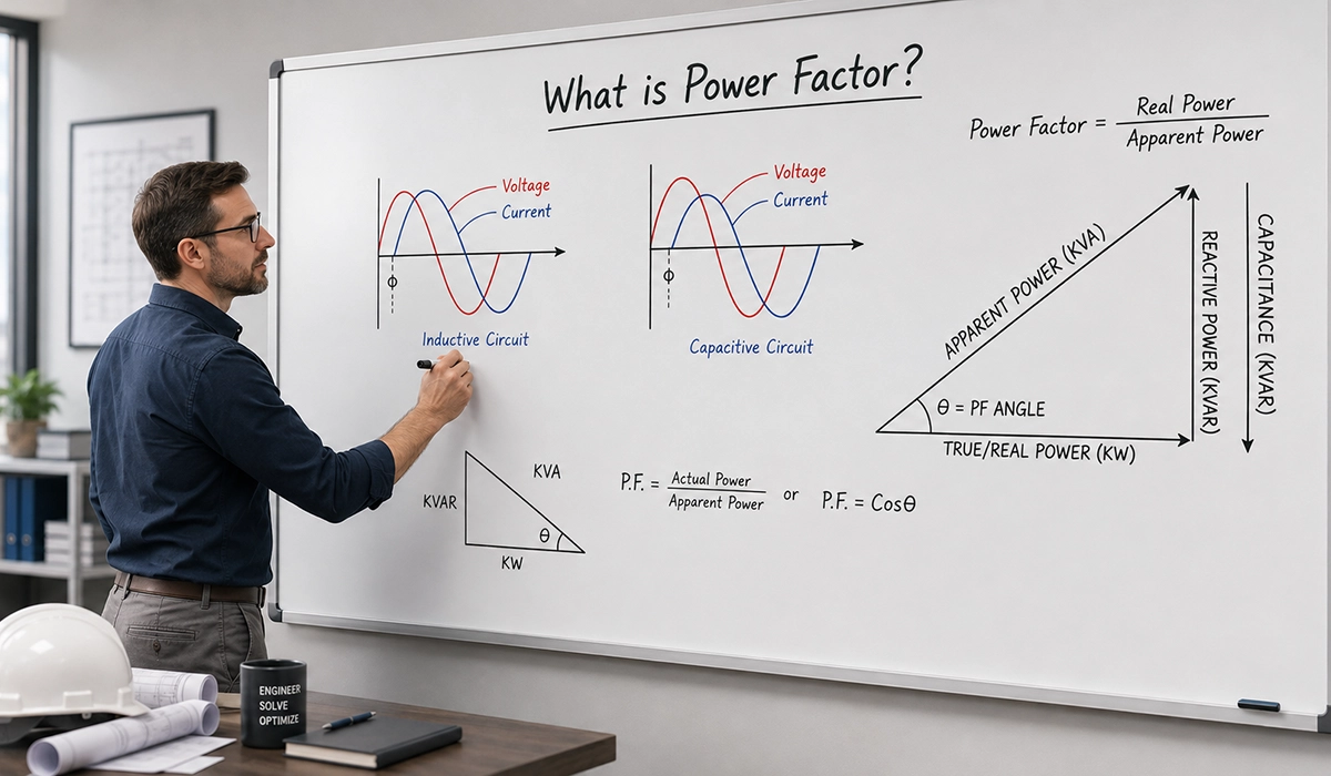
The power triangle gives the kW kVA kVAR relationship a clear geometric form. Engineers draw it as a right-angled triangle with P on the horizontal axis, Q on the vertical axis, and S as the hypotenuse. The angle between P and S is φ, and cos(φ) is the circuit power factor.
The Pythagorean theorem connects the three sides: S² = P² + Q². Therefore S = √(P² + Q²). This compact form proves immediately useful for sizing transformers and selecting correction capacitors.
The triangle also reveals why poor performance is costly. As Q grows, the hypotenuse S stretches even though P stays fixed. Consequently, the supply must deliver more total volt-amperes for the same productive output. Conversely, correction reduces Q, shrinks S, and pulls φ toward zero.
Hence the triangle is not merely academic. It is the engineer’s diagnostic shortcut for visualizing every reactive compensation decision.
Leading vs. Lagging Power Factor
Engineers describe two opposite phase conditions in AC systems. A lagging power factor occurs when inductive loads — motors, transformers, ballasts — delay current behind voltage. This is the dominant condition in industrial plants because inductive load power factor effects usually outweigh capacitive load power factor effects.
By contrast, a leading condition occurs when capacitive elements pull current ahead of voltage. Long unloaded cables, oversized correction banks, and some electronic loads create this state. Leading conditions are less common but cause voltage rise and regulator instability when uncontrolled.
The reactive power direction therefore differs. Lagging loads absorb reactive power from the source. Leading loads return it. Most utility tariffs penalize both extremes, although lagging penalties dominate practical billing.
Furthermore, virtually every industrial correction system targets a slightly lagging condition between 0.95 and 0.99 rather than exact unity. This margin avoids the voltage regulation issues that accompany over-correction while still minimizing reactive demand and cable losses across the plant.
| Condition | Cause | Current vs Voltage | Reactive Power Direction | Common In |
|---|---|---|---|---|
| Lagging PF | Inductive Load | Current Lags Voltage | Source Supplies Q to Load | Motors, Transformers |
| Unity PF | Purely Resistive | In Phase | No Reactive Exchange | Heaters, Incandescent Lamps |
| Leading PF | Capacitive Load | Current Leads Voltage | Load Returns Q to Source | Capacitor Banks, Long Cables |
These formulas change slightly across supply arrangements, so compare single-phase and three-phase power carefully before applying the equations to any industrial distribution board.
What Causes Low Power Factor in Industrial Facilities?
Several recurring drivers explain low power factor causes and effects across factories. Recognizing them is the first step in any audit.
First, induction motors running at partial load dominate the problem. Such motors draw nearly constant magnetizing current regardless of mechanical demand. Therefore a 75 kW motor at 30% load may operate at PF below 0.5. By contrast, the same motor at full load might reach 0.85.
Second, lightly loaded transformers contribute steady magnetizing VAR. Facilities with redundant transformer capacity pay a quiet reactive penalty all day.
Third, older fluorescent lighting with magnetic ballasts still appears in legacy buildings. LED retrofits eliminate this contribution but remain incomplete in many plants.
Fourth, variable frequency drives, UPS systems, and switched-mode supplies inject harmonics. These distort current shape and reduce true power factor even when displacement PF reads acceptable.
Finally, arc welders and arc furnaces draw violent reactive surges. Fixed capacitors cannot follow such fluctuations, so dynamic compensation becomes essential.
Diagnosing these drivers correctly starts with basic circuit theory, and a short refresher on Ohm’s law helps engineers interpret current readings during any plant audit.
The Financial and Operational Consequences of Low Power Factor
Poor performance hits industrial budgets through four channels. Each is measurable, and together they often justify correction within twelve to twenty-four months.
First, the power factor penalty utility tariffs apply bites hardest. Most industrial contracts surcharge facilities below 0.90 or 0.95 PF. Consequently, these add 10–20% to monthly electricity bills in high-demand plants.
Second, oversized infrastructure costs more upfront and across its lifetime. A 500 kW load at 0.75 PF requires 667 kVA of transformer and cable capacity. The same load at 0.95 PF needs only 526 kVA — a 21% reduction in capital outlay.
Third, conductor losses scale with current squared. Reactive current produces real I²R heat that never reaches productive use. Cooling load on switchboards therefore rises in lockstep.
Fourth, voltage drop worsens across long feeders. Sensitive control gear and motor performance suffer accordingly. Hence correction usually improves equipment reliability alongside cutting bills — a benefit operations teams notice quickly.
| Active Power | Power Factor | Apparent Power | Excess kVA vs Unity |
|---|---|---|---|
| 500 kW | 1.00 | 500 kVA | — |
| 500 kW | 0.95 | 526 kVA | +5% |
| 500 kW | 0.90 | 556 kVA | +11% |
| 500 kW | 0.85 | 588 kVA | +18% |
| 500 kW | 0.75 | 667 kVA | +33% |
| 500 kW | 0.65 | 769 kVA | +54% |
Quantifying these losses accurately requires confident use of the electrical power formula, which converts measured voltage and current into the kW and kVA figures tariffs depend on.
Power Factor Correction: Methods and Strategies
Four mainstream power factor correction methods dominate modern facilities. Selection depends on load behavior, harmonic content, and budget.
Fixed capacitor banks suit stable predictable loads where reactive demand changes little across the day. Automatic banks adapt step by step to varying loads and represent the standard industrial choice. Active harmonic filters address both reactive demand and harmonic distortion together. Motor-terminal capacitors place correction at the point of demand for large continuous motors.
Each method has trade-offs in cost, complexity, and effectiveness. The following subsections describe them in turn. Afterwards, a comparison table summarizes the strengths and limitations side by side. Furthermore, hybrid solutions combining passive banks with active filters increasingly appear in plants with heavy VFD content, because neither technology alone covers every operating regime.
Selection should always begin with a power quality survey rather than a generic specification. Site-specific data prevents both under-correction and the over-correction that causes leading PF problems.
Fixed Capacitor Banks
Power factor correction capacitors in fixed banks generate constant leading kVAR that offsets inductive demand. They are the simplest correction form and the most economical. However, sizing must match the lightest operating load to avoid over-correction at night or during shutdowns. Otherwise, a leading condition appears, raising voltage and tripping sensitive equipment.
Automatic (Switched) Capacitor Banks
Automatic panels switch capacitor steps in and out under controller logic. Therefore, the system maintains target PF between 0.95 and 0.99 across the full operating cycle. Industrial plants with variable load profiles almost always specify automatic banks rather than fixed banks because they accommodate production swings cleanly.
Active Power Factor Correction and Harmonic Filters
Active harmonic filters inject counter-phase currents that cancel harmonic distortion in real time. Consequently, they correct true power factor — not just displacement PF. Plants dense with VFDs, UPS systems, and switched-mode loads benefit most. By contrast, passive capacitors can resonate dangerously with harmonics if applied without filtering.
Power Factor Correction at Motor Level
Motor-terminal capacitors correct reactive demand right at the source. Hence cable losses across the entire motor branch fall. This approach suits power factor correction for induction motors running continuously. However, sizing matters: oversized capacitors can cause self-excitation when the motor coasts after de-energising, generating dangerous voltages that damage windings.
| Method | Best For | Advantages | Limitations |
|---|---|---|---|
| Fixed Capacitor Bank | Stable Loads | Simple, Low Cost | No Adaptation; Over-Correction Risk |
| Automatic Capacitor Bank | Variable Loads | Adapts to Demand; Maintains Target | Higher Cost; Needs Controller |
| Active Harmonic Filter | Non-Linear Loads | Corrects Harmonics and PF | Highest Cost; Complex Installation |
| Motor-Level Capacitors | Large Continuous Motors | Reduces Branch Losses | Self-Excitation Risk if Oversized |
What Is a Good Power Factor for an Industrial Facility?
Most utilities set minimum acceptable values between 0.90 and 0.95. Below that threshold, penalties begin. Engineering best practice therefore targets 0.95 to 0.98 lagging as the optimal operating band for industrial sites.
This range avoids utility surcharges and trims infrastructure requirements while staying safely lagging. As a result, the system avoids the voltage regulation issues that accompany leading conditions. Moving above 0.98 is achievable but rarely cost-justified through additional capacitors alone.
Plants dense with VFDs or active front-end converters often reach near-unity inherently. Their drives correct PF internally. By contrast, motor-dominant plants on older infrastructure rarely exceed 0.85 without intervention.
Any reading below 0.85 should trigger an energy audit immediately. The combination of penalties, oversized switchgear, and elevated I²R losses at that level represents recoverable cost that frequently exceeds expectations. Furthermore, a brief power quality study often reveals quick wins worth more than a year of penalty payments.
| PF Range | Assessment | Typical Action |
|---|---|---|
| 0.98 – 1.00 | Excellent | No Correction Needed |
| 0.95 – 0.97 | Good | Meets Most Utility Thresholds |
| 0.90 – 0.94 | Acceptable | Monitor; Correct if Penalised |
| 0.85 – 0.89 | Poor | Correction Recommended |
| Below 0.85 | Very Poor | Correction Required; Penalties Likely |
Conclusion about power factor
Power factor sits at the intersection of physics, billing, and capital planning. Improving it from 0.80 to 0.95 cuts apparent power demand by roughly 16% — meaning smaller transformers, lower bills, cooler cables, and steadier voltage at the point of use.
The path forward is straightforward. Measure first with a recording analyser. Identify whether the issue is displacement, harmonic, or both. Match the correction technology to the load profile. Furthermore, retest after installation to verify that the corrected system avoids the leading condition during off-peak hours.
For most industrial plants, the payback on properly engineered correction falls between twelve and twenty-four months. Hence treating reactive compensation as an energy management priority — rather than a billing nuisance — turns a recurring cost into a one-time investment with measurable returns.


Rate this article
Choose a rating from 1 to 5 stars.
No ratings yet